Hello folks. There’s been some time since I’ve written my last post. I’ve been very busy with work and other side projects, which eventually will find their way here, but since they’re far from completion, I thought to make a smaller post about a subject that is useful and I’ve had had in my notes for a long time. So I figured I’d just put it up on the blog so it could be useful as reference for someone, or even myself one of these days.

The subject is simple, how to tune a dual-band antenna. There’s a fair amount of articles and tutorials, even on YouTube, about matching networks, either LC and Pi networks. They’ll teach you all you need to know about Smith charts and what not. That’s all very useful, but they all have one problem, they usually focus on having impedance $Z_1=R_1+jX_1$ Ω become $Z_0$ Ω at one single frequency. But how do you do it when your antenna is suppose to operate at two different frequency bands? How to tune both bands to 50 Ω (or other complex frequency for that matter)?

It’s rather common if you think about it: WiFi systems operate at 2.4 GHz as well as 5 GHz frequency bands (and now since WiFi 6 has been introduced, the 6 GHz band has been added). So you got to have a frontend that operates in both bands, but you probably only want to use a single antenna for everything. A single antenna that covers the frequency range between 2.4 to 6 GHz is certainly possible, but not at the size you’d appreciate for a small embedded system. Mobile systems also, with GSM/GPRS, UMTS and LTE and now 5G bands coming into place, that’s lot of bands to cram into the smaller number of antennas possible. Small antennas are inherently narrowband, so the only option is to make them operate at the correct bands, to aid it, you have to design appropriate matching networks that make the antenna operate at all those multiple bands, and that means you need to juggle the matching at different frequencies.

Let’s try to make it simple and not delve into the black magic arts… seriously this is engineering!

I’m not going to go over the basic theory of LC matching networks, that can be found in microwave electronics books such as Pozar’s book, or other websites and even YouTube videos, I recommend W2AEW (aka Alan) videos, they’re super, here’s his video about impedance matching networks. There’s even handy calculators out there to help you out, such as this one.

What is lacking in most of these online resources, is that they focus on matching impedance $Z_A$ to impedance $Z_0$ at a single frequency. But when you’re dealing with multiband systems, you need to match two different impedances at two different frequencies to your system reference impedance (usually 50 Ω) . Certainly by learning the theory behind it, especially if you read the book, you can get there. And that’s essentially what I want to cover in this post, how you can use those concepts and apply them to this specific scenario of a dual band antenna.

Let’s take this simple PIFA for our purpose here. A very simple antenna, with regular printed antenna characteristics:

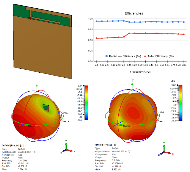
If you notice the efficiencies plot, and as a refresher, the total efficiency is essentially the radiation efficiency minus the losses due to impedance mismatch, you realize the antenna has very good radiation efficiency at both frequency bands, but it suffers from poor impedance matching, which accounts for roughly 30% loss in efficiency. Instead of jeopardizing the radiation efficiency or require more PCB volume for the antenna area, we’ll improve the impedance match using a matching network.

I also took this opportunity to start looking into QucsStudio, which is a free (not open source though) software for circuit simulation, with S-parameter simulation as well as Harmonic Balance simulation capabilities, which allows you to simulate RF circuits in high power regimes, and also some EM (Electromagnetic) simulation capabilities that have been introduced in the latest release. This is extremely useful if you’re designing a power amplifier, for instance, where you want to match your circuit to an input signal with high power, and also check the distortion effects arising from a transistors non-linear behavior. Working on the linear operation zone of a transistor is great, but you’ll not get good efficiencies if you don’t venture into non-linear territory. But that’s talk for another post, in this one, I’ll stick to linear behavior since we’re working with S-parameters only.

NOTE: Antennas are essentially linear devices, but it is not true all the time: A printed antenna will show non-linear behavior if the input signal is large enough. But that occurs essentially due to dielectric breakdown effects and therefore a very high power signal is required to get into that territory, and by very high, I mean hundreds of Watts power range.

Looking at the input impedance of the antenna, we have the following:

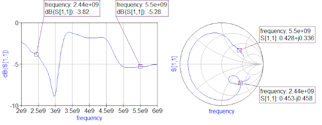
It’s clear that the matching is bad at both bands. Now, the trick to match this impedance, is to first match the lowest band, using only high pass configurations of lumped components, that is, series capacitors and shunt inductors. Series capacitors and shunt inductors are high pass filters, therefore, they’ll play a major role at the lower frequency, but have less influence in the highest band and vice-versa for shunt capacitors and series inductors.

By applying this principle, we can look at the impedance in the Smith chart and trace our course to the center. Following the principle stated previously, we have to navigate by a common admittance circle until we reach the unitary impedance circle by using a shunt inductor (follow the blue curve of the chart on the left) and then follow the common impedance circle with a series capacitor until we reach the center (follow the green curve on the left side chart).

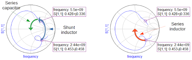
Now, one can wonder, why not simply use a single series inductor, and move directly to the center? We’d save one component and get the same effect. That is correct, if we’re matching only a single band. Using a single shunt capacitor would have a considerable effect on the highest frequency and make it much harder to match in a single shot.

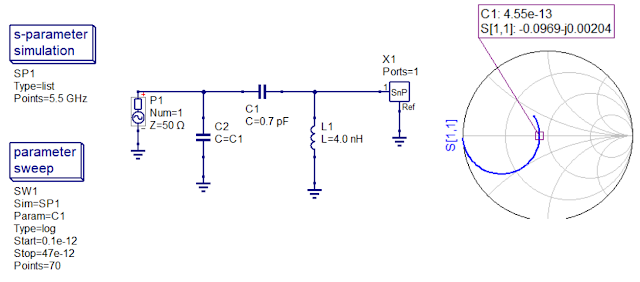
To determine the correct component values you can either calculate them, use an online calculator, or do as I did which is to add one component at the time and do parameter sweeps to the component values. For instance, after adding a shunt inductor to the circuit, like in the picture below. Then by looking at the Smith chart result, we can see that the inductance value of 4.08 nH comes close to the point we want, so I chose 4.0 nH, which is a realistic component value and move on to the series capacitor.

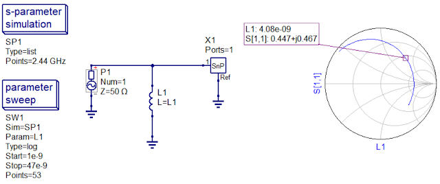
NOTE: The values on the Smith chart are S-parameter values, and not impedance values. In order to get the impedance values, use the math function rtoz(S[1,1], 50), which converts S-parameters to Z-parameters, where the second argument of the function the reference impedance of the system. Here’s a tip, create a table output and use the rtoz( ) function to see the impedance values you get when sweeping the component values.

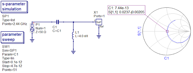
Doing the same as before, but now sweeping the values of the series capacitor, we can reach the center of the Smith chart with a 0.7 pF capacitor. This leads to the following result:

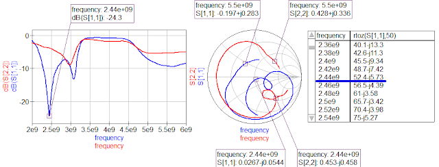
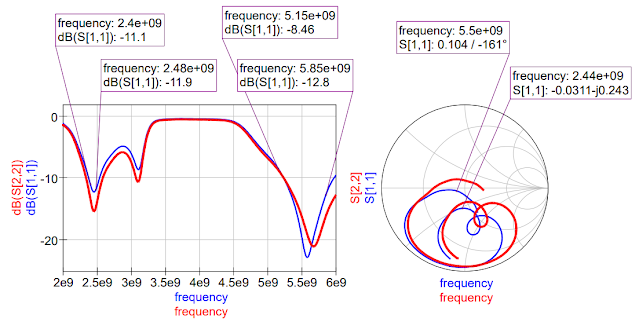
The 2.4 GHz band is done. As you can see, the 5 GHz moved as well, however, it’s movement was small and actually beneficial, since now we can match the 5 GHz band by simply adding a shunt capacitor. Conversely, if we’d use a series inductor, as mentioned above, the 5 GHz band would move to a value with large inductance which would require a series capacitor to match it. But the series capacitor would then move the lowest frequency band away from the tune we’ve reached. The figure below shows the comparison of the low band match between the CL circuit described thus far and the single series inductor.

You can see what I described previously. At 2.4 GHz we get a good match, but at 5.5 GHz the impedance moves to a place where it’s difficult to match without affecting back the lowest band.

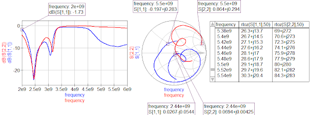
Going back to our circuit, as mentioned above, the thing left to do is to add a shunt capacitor to match the 5 GHz band. Following the same procedure as before, we get to a value of approximately 0.5 pF to match the 5 GHz band.

This circuit, leads us to the following final results (in blue). Which is not bad, but can be improved. If we teak the latest shunt capacitor a bit off the center, by using a 0.3 pF capacitor instead of 0.5 pF, we may get a better match at the 2 GHz band (in red).

Now, this is all good and all, but the truth is, in a real PCB, you have tracks in between the components, and these are not ideal, they have parasitics due to the nature of their packages, as well as parasitics which are formed between them and the PCB tracks. All these effects are considerable at GHz frequencies and they’ll impact the matching. If one simulates the circuit behavior in such a manner, it will fail miserably in a real application. But I’ll leave a demonstration of such scenario for my next post (which I seriously hope won’t take so long).

That’s all for today.

Stay tuned (in whatever bands you want)!